LYFTOFF v3.0LYFTOFF v3.0 - Complete Professional Trading System
Educational Indicator - Not Financial Advice
This indicator is provided for educational purposes only. It does not constitute financial, investment, or trading advice. Past performance does not guarantee future results. Trading involves substantial risk of loss. You are solely responsible for your trading decisions. Always consult a licensed financial advisor before making investment decisions.
━━━━━━━━━━━━━━━━━━━━━━━━━━━━━━━━━━
Introducing LYFTOFF v3.0
━━━━━━━━━━━━━━━━━━━━━━━━━━━━━━━━━━
Most traders fail because they're overwhelmed. Most indicators give you a buy signal and leave you stranded. Where's my stop loss? Should I take profit? When do I exit? You're on your own. 47 indicators giving conflicting signals. No idea which ticker to trade, when to enter, where to set stops, when to take profit, when to exit. Trading becomes stressful and exhausting. They quit.
LYFTOFF changes this. From the moment you install it: tells you which tickers to trade, shows when conditions are ideal, gives multiple entry options, sets stop loss automatically, warns about risk and volatility, tracks institutional positioning, takes profits systematically, exits before crashes, tracks performance. Now retail traders have institutional-grade trade management without institutional fees.
What Makes LYFTOFF Unique
Asset-Class Optimization - Different settings for stocks vs crypto vs sectors.
3D Ticker Health Analysis - Dashboard synthesizes 8 factors into one color-coded view.
Risk-Calibrated Entry Strategies - 4 different entry types for different risk tolerances.
Continuous Position Management - Stop Loss tracking, Volatility warnings, Risk assessment, Profit-taking.
Inverse Chart Institutional Tracking - Analyzes 1/ticker to detect when institutions accumulate during panic.
Intelligent Profit-Taking - Trim signals based on meaningful profit thresholds with exact PNL%.
Comprehensive Labeling - All signals show exact prices, dynamic PNL%, stop levels.
Complete Accessibility - Colorblind mode, full functionality available to all users.
LYFTOFF guides you through the entire trade lifecycle.
━━━━━━━━━━━━━━━━━━━━━━━━━━━━━━━━━━
Step 1: The Trading Lifecycle - Which ticker should I trade?
━━━━━━━━━━━━━━━━━━━━━━━━━━━━━━━━━━
Scan multiple tickers and identify which ones are performing best with LYFTOFF signals.
Rate of Return Display (bottom right corner)
Tracks actual performance over past 52 weeks based on completed buy to short trades. Shows one of three ratings:
- High Return (green) = 15%+ compounded gains - Trade this ticker
- Moderate Return (yellow) = 5-15% compounded gains - Acceptable ticker
- Low Return (red) = Under 5% compounded gains - Avoid this ticker
━━━━━━━━━━━━━━━━━━━━━━━━━━━━━━━━━━
Step 2: The Trading Lifecycle - How do I optimize for this asset class?
━━━━━━━━━━━━━━━━━━━━━━━━━━━━━━━━━━
Customize LYFTOFF for different asset classes.
LYFTOFF Profit Optimizer
Asset-class-specific settings automatically applied:
- Stocks & ETFs - Optimized for indices and broad market
- Crypto - Optimized for Bitcoin, Ethereum, blockchain assets
- Market Sectors - Optimized for high-growth sector ETFs
━━━━━━━━━━━━━━━━━━━━━━━━━━━━━━━━━━
Step 3: The Trading Lifecycle - Is this a good opportunity?
━━━━━━━━━━━━━━━━━━━━━━━━━━━━━━━━━━
One glance shows complete market health. No other indicator provides this.
LYFTOFF Dashboard
8-row color-coded table (top right):
1. Trend - Direction
2. Timing - Entry quality
3. Momentum - Underlying strength
4. Strength - Price action power
5. Speed - Trend acceleration
6. Risk - Safety conditions
7. Volatility - Market stability
8. Inverse Chart - Institutional positioning
━━━━━━━━━━━━━━━━━━━━━━━━━━━━━━━━━━
Step 4: The Trading Lifecycle - What's my risk tolerance?
━━━━━━━━━━━━━━━━━━━━━━━━━━━━━━━━━━
Four Entry Strategies
1. Gold Setup (Ultra-Conservative)
All three systems aligned: Trend + Institutions + Safety
Rarest signal. Highest probability. 1-3 per year.
2. Buy Setup (Conservative)
Confirmed uptrend with trailing stop loss
Primary entry signal.
3. Trend Change Early Warning (Moderate Risk)
Momentum shifting before trend confirms
Buy Setup typically follows in 1-4 weeks.
4. Buy the Dip Setup (Aggressive - High Risk/Reward)
Extreme oversold + extreme volatility
Catch the exact bottom.
━━━━━━━━━━━━━━━━━━━━━━━━━━━━━━━━━━
Step 5: The Trading Lifecycle - What's happening? What should I do?
━━━━━━━━━━━━━━━━━━━━━━━━━━━━━━━━━━
Continuous Guidance
Stop Loss Label
Exact price level. Updates as trend continues.
Volatility Regime (above candles)
- Low Volatility - Full position size safe
- Medium Volatility - Reduce to 50% size
- High Volatility - Protect capital
Shows duration + current PNL%
Safe Signal (bottom chart - colored arrows)
Green = Safe | Yellow = Caution | Orange = Danger | Red = Extreme oversold
Super Safe Triangles (near candles)
Green = Institutions accumulating | Red = Institutions distributing
Uses inverse chart analysis (1/ticker)
Trim Alert
Shows "Trim Alert" + price + PNL% when position has meaningful profit
Lock in 25-50% gains.
━━━━━━━━━━━━━━━━━━━━━━━━━━━━━━━━━━
Step 6: The Trading Lifecycle - When do I sell?
━━━━━━━━━━━━━━━━━━━━━━━━━━━━━━━━━━
Short Setup
Clear exit signal when trend breaks. Exit to cash.
━━━━━━━━━━━━━━━━━━━━━━━━━━━━━━━━━━
7 Configurable Alerts
━━━━━━━━━━━━━━━━━━━━━━━━━━━━━━━━━━
1. 'Buy (Low Risk Trade)'
2. 'Short (Low Risk Trade)'
3. 'Stop Loss (Price crossed below stop)'
4. 'Buy the Dip (High Risk Trade)'
5. 'Trim (No Risk Trade)'
6. 'Trend Change (Bullish Trend Change)'
7. 'Gold Setup (Low Risk Trade)'
Set to "Once Per Bar Close" for weekly charts.
━━━━━━━━━━━━━━━━━━━━━━━━━━━━━━━━━━
Weekly Timeframe - Why It's Optimal
━━━━━━━━━━━━━━━━━━━━━━━━━━━━━━━━━━
LYFTOFF is optimized for weekly (1W) charts:
- Filters out noise and false signals
- Aligns with institutional timeframes
- Lower transaction costs
- Time freedom (5 min Sunday, 2 min Monday, 0 min rest of week)
- 3-5 high-probability setups per year
Signals have not been validated outside weekly timeframe.
━━━━━━━━━━━━━━━━━━━━━━━━━━━━━━━━━━
Known Limitations
━━━━━━━━━━━━━━━━━━━━━━━━━━━━━━━━━━
Technical:
Free accounts may have issues with Super Safe triangles | Gold Setup only on Daily/Weekly timeframes | Many labels on long historical charts
Strategic:
Trend-following system underperforms in choppy markets | Signals appear after trend changes begin (by design) | Whipsaw risk in volatile markets | 3-5 setups per year (not for active traders)
Market Conditions:
Bull market bias (1995-2025 backtesting period) | May fail during black swan events | Crypto shows exceptional returns but higher risk
━━━━━━━━━━━━━━━━━━━━━━━━━━━━━━━━━━
How to Use
━━━━━━━━━━━━━━━━━━━━━━━━━━━━━━━━━━
Setup:
1. Select asset class in Profit Optimizer
2. Set chart to Weekly (1W)
3. Configure 7 alerts ("Once Per Bar Close")
4. Enable notifications
Weekly Routine:
Sunday (5 min) - Check for signals
Monday (2 min) - Execute trades if signals appeared, set stop loss
Tuesday-Saturday - Do nothing
Signal Actions:
Buy Setup - Enter long | Short Setup - Exit to cash | Buy the Dip - Conservative: wait; Aggressive: enter with tight stop | Trend Change - Watchlist | Trim - Sell 25-50% | Gold Setup - Maximum conviction | Stop Loss - Exit if crossed
Risk Management:
Risk 2-5% per trade maximum | Honor all stop losses | Never hold past Short Setup | Start small, scale after 10+ trades
━━━━━━━━━━━━━━━━━━━━━━━━━━━━━━━━━━
Vendor Information
━━━━━━━━━━━━━━━━━━━━━━━━━━━━━━━━━━
Author: REGGAWAVE LLC | Version: 3.0 | License: Mozilla Public License 2.0
Copyright: 2026 REGGAWAVE LLC. All Rights Reserved.
Proprietary intellectual property. Unauthorized copying, modification, or distribution prohibited.
Support: TradingView comment system on this publication.
User Agreement:
By using this indicator, you acknowledge you accept full responsibility for trading decisions, understand substantial risk is involved, REGGAWAVE LLC provides no warranties or guarantees, REGGAWAVE LLC is not liable for losses, this is educational content not financial advice, and REGGAWAVE LLC is not a registered investment advisor.
2026 REGGAWAVE LLC. All Rights Reserved.
Pine Script®指标